Lighting in OpenGL

Color

We all know that the reason human eyes can see things is due to two situations:

1. We see the light emitted by the object.
2. The object reflects the light emitted by a luminous object.

Every object has a different color because they have different reflection capabilities for light. For example, leaves reflect the green light from the white light emitted by the sun, and the human eye receives this light, thus perceiving the leaves as green. If the leaves are placed under red light, they will absorb all light except for green light, appearing black.

The ability of an object to reflect a certain color is called reflectance.

If we use a three-dimensional vector to describe the color of light, then after reflection, one component of the object's color equals the corresponding component of the light source multiplied by the object's reflectance for that color component.

Basic Lighting

Lighting in displays is extremely complex and influenced by many factors, which our limited computational capabilities cannot simulate.

Therefore, OpenGL uses a simplified model for lighting, approximating real-world situations, making it easier to handle while still looking quite similar. These lighting models are based on our understanding of the physical properties of light. One of the models is called the Phong Lighting Model.

The Phong lighting model mainly consists of three parts:

• Ambient
• Diffuse
• Specular

Material

In the real world, each object reacts differently to light. For example, steel objects usually appear shinier than clay vases, and a wooden box will not reflect the same amount of light as a steel box. Some objects reflect light with minimal scattering, resulting in smaller specular highlights, while others scatter a lot, producing larger specular highlights. If we want to simulate various types of objects in OpenGL, we must define different material properties for each surface.

In the following code, we define a material by setting diffuse and specular maps.

struct Material {
    sampler2D diffuse;
    sampler2D specular;    
    float shininess;
}; 

By using diffuse and specular maps, we can add a lot of detail to relatively simple objects. We can even use normal/bump maps or reflection maps to add even more detail to the objects.

Light Sources

Directional Light

When a light source is very far away, the rays from the light source will approximate parallelism. Regardless of the position of the object and/or observer, it appears that all light comes from the same direction. When we use a model that assumes the light source is infinitely far away, it is referred to as directional light, because all its rays have the same direction, and its position does not matter.

A great example of directional light is the sun. The sun is not infinitely far from us, but it is far enough that we can treat it as infinitely distant in lighting calculations. Thus, all rays from the sun will be simulated as parallel rays.

Point Light

Directional light is excellent for illuminating the entire scene as a global light source, but in addition to directional light, we also need some point lights scattered throughout the scene. A point light is a light source located at a specific position in the world, emitting light in all directions, but the intensity of the light diminishes with distance. Imagine a light bulb or a torch; they are both point lights.

Light Attenuation

The gradual reduction of light intensity as the light travels further is commonly called attenuation. One way to reduce light intensity with distance is to use a linear equation. Such an equation can linearly decrease the intensity of light as distance increases, making distant objects appear darker. However, such a linear equation often looks unrealistic. In the real world, lights are usually very bright up close, but as the distance increases, the brightness of the light source initially drops quickly, but at greater distances, the remaining intensity decreases very slowly. Therefore, we need a different formula to reduce light intensity.

where the constant term $K_c$, the linear term $K_l$, and the quadratic term $K_q$ are customizable.

• The constant term is usually kept at 1.0, primarily to ensure that the denominator never becomes less than 1; otherwise, at certain distances, it would increase intensity, which is definitely not the desired effect.
• The linear term will multiply with the distance value to reduce intensity linearly.
• The quadratic term will multiply with the square of the distance, allowing the light source to decrease intensity quadratically. The quadratic term has a much smaller effect when the distance is small, but it becomes larger than the linear term when the distance value is large.

Spotlight

A spotlight is a light source located at a certain position in the environment that only emits light in a specific direction rather than all directions. As a result, only objects within a specific radius in the direction of the spotlight will be illuminated, while others remain dark. Good examples of spotlights are streetlights or flashlights.

In OpenGL, a spotlight is represented by a world space position, a direction, and a cutoff angle, which specifies the radius of the spotlight (note: this is the radius of the cone, not the distance from the light source). For each fragment, we calculate whether the fragment is within the cutoff direction of the spotlight (i.e., within the cone), and if so, we illuminate the fragment accordingly.

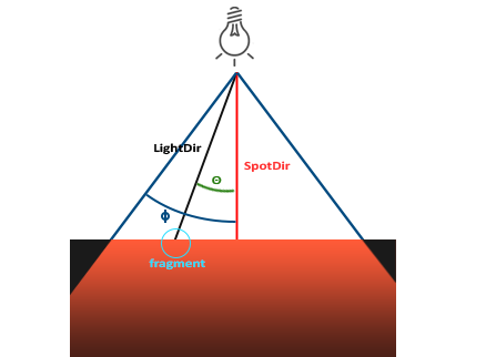
• LightDir: The vector from the fragment to the light source
• SpotDir: The direction of the spotlight
• $\phi$: The cutoff angle that specifies the radius of the spotlight. Objects outside this angle will not be illuminated by the spotlight.
• $\theta$: The angle between the LightDir vector and the SpotDir vector. The $\theta$ value inside the spotlight should be smaller than the $\phi$ value.

Smooth Edges

We can achieve a soft edge effect by defining two cutoff angles, and creating a gradient between these two angles. We can use this formula to calculate this value:

Here, $\epsilon$ (Epsilon) is the difference in cosine values between the inner ($\phi$) and outer cones ($\gamma$) ($\epsilon=\phi-\gamma$). The final $I$ value represents the intensity of the spotlight at the current fragment.

Let’s explain how this function works. Since the inner and outer angles need to be between $(0,\frac{\pi}{2})$, the cosine function is monotonically decreasing in this range. Because the inner angle $\phi$ and the outer angle $\gamma$ are fixed, as the incident angle $\theta$ moves from vertical to horizontal, i.e., from 0 to $\frac{\pi}{2}$, $cos(\theta)$ decreases monotonically. This value is maximum when $\theta=0$, starts to be less than 1 when $\theta>\phi$, equals 0 when $\theta=\gamma$, and becomes negative when greater than $\gamma$. If we use a clamping function to restrict the function value within the range $[0,1]$, it can represent full brightness within the inner angle, complete darkness outside the outer angle, and a smooth decrease in light intensity between the two cutoff angles.

Normal Matrix

How does a fragment's normal change during model transformation? If the fragment undergoes normal rotation or translation, the normal can simply undergo the same operation. Additionally, if the fragment undergoes uniform scaling (the scaling factor is the same for each component), the normal also only needs to undergo the same operation.

However, there is a special case where, when the fragment undergoes non-uniform scaling, the normal cannot simply undergo the same operation. The following image illustrates why this cannot be done:

It is clear that the second normal is no longer perpendicular to the plane, and we can solve this problem using the normal matrix.

The normal matrix is the inverse transpose matrix of the model matrix. That is, $M_n=(M^{-1})^T$.

Why the Inverse Transpose Matrix

Assuming we need a transformation matrix $A$ to transform the original normal vector $n$ into a vector $n^{'}$ that is perpendicular to the transformed fragment's tangent $t$, we have $n\cdot t=0$. After transformation, the tangent becomes $Mt$, so we need $n^{'}\cdot (Mt)=0$.

Thus, we have:

.

Using the dot product, we get:

Since the initial condition $n^Tt=0$ holds for all tangents $t$, we have $A^TM=I$, where $I$ is the identity matrix.

We can solve for:

Therefore, the normal matrix must be the inverse transpose matrix of the model matrix. Calculating the inverse transpose of a matrix is an expensive operation, so it should only be computed when the fragment undergoes non-uniform scaling and when $M$ is not an orthogonal matrix ($M^{-1}\neq M^T$).