What is OpenGL?

As mentioned in the ArcVP Development Log, in short, OpenGL is a standard for a graphics API. Each graphics card manufacturer implements its own version of OpenGL, similar to the relationship between the C++ standard and different compilers.

Core Profile vs. Immediate Mode

Early versions of OpenGL used Immediate Mode (fixed-function pipeline), which made drawing graphics very convenient. Most of OpenGL's functionality was hidden behind libraries, giving developers little freedom to control how OpenGL performed calculations. Developers were eager for more flexibility. Over time, the specification became more flexible, allowing developers more control over drawing details. While Immediate Mode is indeed easy to use and understand, it is inefficient. Therefore, starting from OpenGL 3.2, the specification began to deprecate Immediate Mode and encouraged developers to develop under OpenGL's Core Profile, which completely removed the old features.

When using OpenGL's Core Profile, OpenGL forces us to use modern functions. When we attempt to use a deprecated function, OpenGL throws an error and terminates the drawing. The advantage of modern functions is higher flexibility and efficiency, but they are also harder to learn. Immediate Mode abstracts away many details of how OpenGL actually operates, making it easy to learn but difficult to grasp how OpenGL works in practice. Modern functions require users to truly understand OpenGL and graphics programming, which can be challenging but offers more flexibility, higher efficiency, and, importantly, a deeper understanding of graphics programming.

This is why our tutorial is aimed at OpenGL 3.3's Core Profile. Although it is more difficult to get started, this effort is worthwhile.

Today, higher versions of OpenGL have been released (the latest version at the time of writing is 4.5). You may ask: since OpenGL 4.5 is out, why should we still learn OpenGL 3.3? The answer is simple: all higher versions of OpenGL are built on the foundation of 3.3, introducing additional features without changing the core architecture. New versions simply provide more efficient or useful ways to achieve the same functionality. Therefore, all concepts and techniques remain consistent across modern OpenGL versions. When you have enough experience, you can easily utilize new features from higher versions of OpenGL.

GLAD

Since OpenGL is just a standard/specification, the actual implementation is done by driver developers for specific graphics cards. Due to the numerous versions of OpenGL drivers, the locations of most functions cannot be determined at compile time and need to be queried at runtime. Thus, the task falls on developers, who need to obtain function addresses at runtime and store them in function pointers for later use. GLAD is a library designed to simplify this process.

Shaders

Shaders are programs that can run on the GPU. There are many types of shaders, each concerned with a small part of the rendering or computation process. A large number of shader instances can run simultaneously on the GPU, and some shaders are programmable. Generally, the input of one type of shader is usually the output of another type of shader. The blue ones below are programmable shaders.

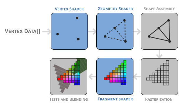
Vertex Shader

The Vertex Shader is one of several programmable shaders. If we intend to render, modern OpenGL requires us to set up at least one vertex shader and one fragment shader. It processes the data for each vertex (such as position, normal, texture coordinates, etc.), transforming vertices from model coordinates to screen coordinates and performing other vertex-related transformations. Generally, the vertex shader transforms points in space to a 2D plane.

Geometry Shader

The output of the vertex shader stage can be optionally passed to the Geometry Shader. The Geometry Shader takes a set of vertices as input, which form primitives, and can generate new shapes by emitting new vertices to form new (or other) primitives.

Primitive Assembly

The Primitive Assembly stage takes all vertices output from the vertex shader (or geometry shader) as input (if it is GL_POINTS, then it is a single vertex) and assembles all points into the shape of the specified primitive. The output of the primitive assembly stage is passed to the Rasterization Stage, where it maps the primitives to the corresponding pixels on the final screen, generating fragments for use by the Fragment Shader. Clipping is performed before the fragment shader runs. Clipping discards all pixels outside your view to improve execution efficiency.

Fragment Shader

The Fragment Shader is typically used to combine textures, perform lighting calculations, shadow effects, and other information to generate the final color of each pixel.

Once all corresponding color values are determined, the final object will be passed to the last stage, which we call the Alpha Testing and Blending stage. This stage checks the corresponding depth (and stencil) values of the fragments to determine whether this pixel is in front of or behind other objects, deciding whether it should be discarded. This stage also checks the alpha value (which defines the transparency of an object) and performs blending. Therefore, even if a pixel's output color is calculated in the fragment shader, the final pixel color may be completely different when rendering multiple triangles.

Shader Program

A shader program can contain the series of shaders mentioned above. We can attach multiple shaders to a program and then perform a link operation to generate a shader program pipeline.

Vertex Input

Before drawing, we need to provide OpenGL with some vertex coordinates. These coordinates need to be within the range of [-1~1], known as Normalized Device Coordinates. Only vertices within this range will ultimately be displayed on the screen. This coordinate system can be understood as a Cartesian coordinate system with the window center as the origin.

Once your vertex coordinates have been processed in the vertex shader, they should be in Normalized Device Coordinates, which is a small space where x, y, and z values range from -1.0 to 1.0. Any coordinates that fall outside this range will be discarded/clipped and will not be displayed on your screen.

Using the data provided by the glViewport function for viewport transformation, we can convert Normalized Device Coordinates into Screen Space Coordinates, which are then transformed into fragments sent to the fragment shader.

Vertex Array

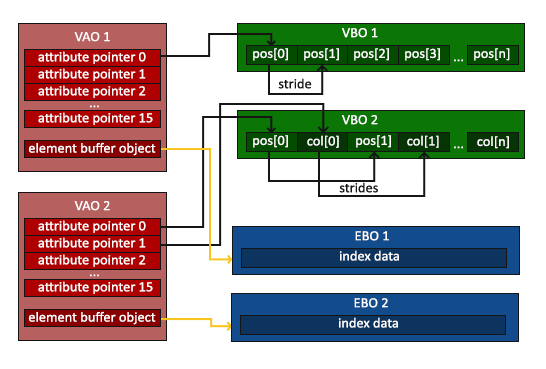The above image shows the relationship between Vertex Array, Vertex Buffer, and Element Buffer. A Vertex Array is an abstraction of all the vertex attributes we use, which can contain multiple Attribute Pointers pointing to specific data in the Vertex Buffer that describes the attributes of a vertex.

Using a buffer instead of individual vertices ensures that they are typically sent to the GPU's memory all at once. Sending data from the CPU to the GPU is a slow process, so we need to send as much data as possible at once.

The Element Buffer is a buffer, similar to the Vertex Buffer, that stores the indices OpenGL uses to determine which vertices to draw. This so-called indexed drawing is the solution to our problem.

Textures

Textures can be simply understood as the images used in a game. We will seamlessly wrap them onto models to create complex appearances.

We can use the fragment shader to work with textures. First, we create and bind the texture, then specify its format and set the data.

A common pitfall when reading texture data is that image data generally uses the top-left corner as the origin, while OpenGL textures use the bottom-left corner as the origin. Using them directly can result in the image being upside down, so we need to flip the image data vertically when reading it.

Texture Filtering

When we apply a texture to a surface of a different size, scaling occurs. We can set different texture filtering methods to achieve different scaling effects. For example, using GL_LINEAR allows for linear interpolation, while GL_NEAREST performs nearest-neighbor sampling.

Mipmap

Using the full texture for a very small surface can lead to excessive overhead. OpenGL provides a solution called mipmap.

It can be understood as pre-created textures of different sizes. For example, if you provide a 500x500 texture, using mipmap, OpenGL can pre-create 200x200 and 50x50 textures. When we apply the texture to a small object, we can directly use the 50x50 variant, reducing computational overhead. Similarly, we can use GL_NEAREST_MIPMAP_LINEAR to specify which mipmap variant to use.

Transformations

Here we need to introduce some basic linear algebra:

Matrix Multiplication

Matrix and Matrix

Assuming we denote a matrix with x rows and y columns as $M_{x,y}$, the multiplication of matrix $M_{m,n}$ and $M_{p,q}$ requires that $n=p$, resulting in $M_{m,q}$.

Moreover, matrix multiplication does not satisfy the commutative property, i.e., $A\cdot B \neq B \cdot A$.

Below is a simple implementation of matrix multiplication.

template <typename T> using mat = std::vector<std::vector<T>>;
mat<int> matrix_multiply(mat<int> const &lhs, mat<int> const &rhs) {
    // Check if matrices are empty
    if (lhs.empty() || rhs.empty() || lhs.front().empty() ||
        rhs.front().empty()) {
        throw std::runtime_error("empty matrix");
    }
    // Dimensions
    int m = lhs.size();         // rows of lhs
    int n = lhs.front().size(); // columns of lhs
    int p = rhs.size();         // rows of rhs
    int q = rhs.front().size(); // columns of rhs
    // Check compatibility: n must equal p
    if (n != p) {
        throw std::runtime_error("matrix dimensions incompatible");
    }
    // Check consistency of inner vector sizes
    for (const auto &row : lhs) {
        if (row.size() != n)
            throw std::runtime_error("inconsistent lhs column sizes");
    }
    for (const auto &row : rhs) {
        if (row.size() != q)
            throw std::runtime_error("inconsistent rhs column sizes");
    }
    // Result matrix: m × q
    mat<int> ret(m, std::vector<int>(q, 0));
    // Matrix multiplication
    for (int i = 0; i < m; i++) {
        for (int j = 0; j < q; j++) {
            for (int k = 0; k < n; k++) { // Use n (or p, since n == p)
                ret[i][j] += lhs[i][k] * rhs[k][j];
            }
        }
    }
    return ret;
}

Matrix and Vector

Similarly, we can assume an n-dimensional vector as a $M_{n,1}$ for performing multiplication between matrices and vectors.

But why do we care whether a matrix can multiply a vector? Well, many interesting 2D/3D transformations can be encapsulated in a matrix, and multiplying this matrix by our vector will transform (Transform) the vector. If you are still a bit confused, let's look at some examples, and you'll understand quickly.

Identity Matrix

The Identity Matrix is a matrix that has all zeros except for the diagonal. Using the identity matrix as a transformation matrix leaves a vector completely unchanged:

Scaling

OpenGL typically operates in 3D space. For 2D situations, we can scale the z-axis by 1, so the z-axis value remains unchanged. The scaling operation we just performed is non-uniform scaling because the scaling factors for each axis are different. If the scaling factors for each axis are the same, it is called uniform scaling. The following transformation matrix can scale a vector by different degrees:

Note that the fourth scaling vector remains 1, as scaling the w component in 3D space is meaningless. The w component has other uses, which we will see later.

Translation

Translation is the process of adding another vector to the original vector to obtain a new vector at a different position, thereby moving the original vector based on the translation vector. We have already discussed vector addition, so this should not be too unfamiliar.

With the translation matrix, we can move objects in the three directions (x, y, z). It is a very useful transformation matrix in our toolbox.

Rotation

Rotating in 3D space requires defining an angle and a rotation axis (Rotation Axis). An object will rotate around the given rotation axis by a specified angle. If you want a more visual understanding, try looking down at a specific rotation axis while rotating your head by a certain angle. When a 2D vector rotates in 3D space, we set the rotation axis as the z-axis (try to imagine this situation). The rotation matrix has different definitions for each unit axis in 3D space, with the rotation angle represented by $\theta$:

Using the rotation matrix, we can rotate any position vector around a unit rotation axis. We can also combine multiple matrices, such as rotating around the x-axis first and then the y-axis. However, this can quickly lead to a problem known as gimbal lock. We will not discuss its details here, but for rotations in 3D space, a better model is to rotate around any arbitrary axis, such as a unit vector $(0.662, 0.2, 0.7222)$, rather than combining a series of rotation matrices.

The real solution to avoid gimbal lock is to use quaternions, which are not only safer but also more efficient in computation.

Matrix Composition

With the different transformation matrices introduced above, we can perform arbitrary transformations on a vector in space. Based on matrix multiplication, we can combine multiple transformation matrices into one matrix.

Coordinate Spaces

The process of transforming coordinates into normalized device coordinates and then into screen coordinates is typically done in steps, similar to a pipeline. In the pipeline, the vertices of an object are transformed into multiple coordinate systems before being finally converted to screen coordinates. The advantage of transforming the object's coordinates into several intermediate coordinate systems is that some operations or calculations are more convenient and easier in these specific coordinate systems, which will soon become apparent. There are a total of five different coordinate systems that are important to us:

• Local Space (also known as Object Space)
• World Space
• View Space (also known as Eye Space)
• Clip Space
• Screen Space

To transform coordinates from one coordinate system to another, we need several transformation matrices, the most important of which are the Model, View, and Projection matrices. Our vertex coordinates start in Local Space, where they are called Local Coordinates. They will then transform into World Coordinates, View Coordinates, Clip Coordinates, and finally end in Screen Coordinates. The following diagram illustrates the entire process and what each transformation does:

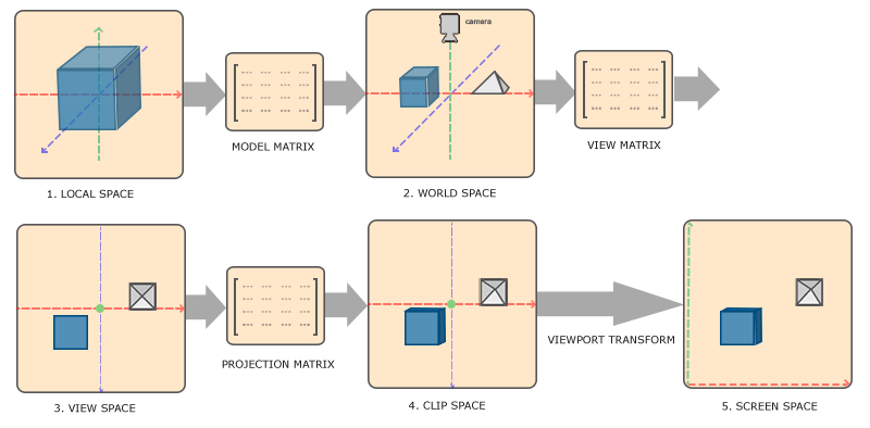
1. Local coordinates are the coordinates of the object relative to its local origin, which is also the starting coordinates of the object.
2. The next step is to transform the local coordinates into world space coordinates, which are in a larger spatial range. These coordinates are relative to the global origin of the world, and they will be placed relative to the world origin along with other objects.
3. Next, we transform the world coordinates into view space coordinates, so that each coordinate is observed from the perspective of the camera or observer.
4. After reaching the view space, we need to project them into clip coordinates. Clip coordinates will be processed to fall within the range of -1.0 to 1.0, determining which vertices will appear on the screen.
5. Finally, we transform the clip coordinates into screen coordinates using a process called Viewport Transform. The viewport transform converts coordinates in the range of -1.0 to 1.0 to the coordinate range defined by the glViewport function. The resulting coordinates will then be sent to the rasterizer, which converts them into fragments.

Local Space

Local space refers to the coordinate space where the object is located, that is, the place where the object initially exists. Imagine you create a cube in a modeling software (like Blender). The origin of the cube you create may be at (0, 0, 0), even though it may ultimately be in a completely different position in the program. It is even possible that all the models you create start at the initial position of (0, 0, 0) (note: however, they will eventually appear at different positions in the world). Therefore, all the vertices of your model are in local space: they are all local relative to your object.

World Space

If we import all objects into the program, they may all be crowded at the world origin (0, 0, 0), which is not the result we want. We want to define a position for each object so that we can place them in a larger world. The coordinates in world space are as the name suggests: they are the coordinates of the vertices relative to the (game) world. If you want to spread objects around the world (especially in a very realistic way), this is the space you want the objects to transform into. The coordinates of the objects will transform from local to world space; this transformation is implemented by the Model Matrix.

The Model Matrix is a transformation matrix that can position an object where it should be by translating, scaling, and rotating it. You can think of it as transforming a house; you need to scale it down (it is too large in local space), move it to a small town in the suburbs, and then rotate it a bit on the y-axis to match the nearby houses. You can also think of the matrix used to place the box around the scene in the previous section as a model matrix; we transformed the local coordinates of the box to different positions in the scene/world.

View Space

View Space is often referred to as OpenGL's Camera (hence sometimes called Camera Space or Eye Space). View Space is the result of transforming world space coordinates into coordinates that are in front of the user's field of view. Thus, view space is the space observed from the perspective of the camera. This is typically accomplished by a combination of translations and rotations, translating/rotating the scene so that specific objects are transformed in front of the camera. These combined transformations are usually stored in a View Matrix, which is used to transform world coordinates into view space. In the next section, we will delve into how to create such a view matrix to simulate a camera. When we multiply the model, view, and projection matrices together and then multiply the resulting matrix by a vector, the result is the corresponding vector in clip space. However, the effect of this matrix product on the vector is applied in reverse order. That is, the multiplication of $model * view * projection$ with the vector is equivalent to first applying the projection transformation to the vector, rather than the model transformation. This result does not meet expectations, so we need to multiply them in reverse order, i.e., $projection * view * model$.

Clip Space

At the end of a vertex shader run, OpenGL expects all coordinates to fall within a specific range, and any points outside this range should be clipped. Clipped coordinates will be ignored, so the remaining coordinates will become the visible fragments on the screen. This is also the origin of the name Clip Space.

To transform vertex coordinates from view space to clip space, we need to define a Projection Matrix, which specifies a range of coordinates, such as -1000 to 1000 in each dimension. The projection matrix will then transform the coordinates within this specified range into normalized device coordinates ranging from -1.0 to 1.0. Any coordinates outside this range will not be mapped to the range of -1.0 to 1.0 and will thus be clipped. Within the range specified by the above projection matrix, the coordinate (1250, 500, 750) will be invisible because its x-coordinate exceeds the range, and it will be transformed into a normalized device coordinate greater than 1.0, so it gets clipped.

If only part of a primitive, such as a triangle, exceeds the clipping volume, OpenGL will reconstruct the triangle into one or more triangles to fit within this clipping range.

The Viewing Box created by the projection matrix is called a Frustum, and every coordinate that appears within the frustum will ultimately appear on the user's screen. The process of transforming coordinates within a specific range into normalized device coordinates (and easily mapping them to 2D view space coordinates) is called Projection, because using the projection matrix allows us to project (Project) 3D coordinates into the easily mappable 2D normalized device coordinate system.

Once all vertices are transformed into clip space, the final operation—Perspective Division—will be executed. In this process, we divide the x, y, and z components of the position vector by the homogeneous w component of the vector; perspective division is the process of transforming 4D clip space coordinates into 3D normalized device coordinates. This step will be automatically executed at the end of each vertex shader run.

After this stage, the final coordinates will be mapped into screen space (using the settings in glViewport) and transformed into fragments.

The projection matrix that transforms view coordinates into clip coordinates can take two different forms, each defining a different frustum. We can choose to create either an Orthographic Projection Matrix or a Perspective Projection Matrix.

Orthographic Projection

The frustum defined by the orthographic projection matrix is similar to a cube, requiring knowledge of its length, width, and height. Only coordinates within this container will not be clipped. The orthographic frustum directly maps all coordinates inside the frustum to normalized device coordinates because the w component of each vector is unchanged; if the w component equals 1.0, the perspective division will not change this coordinate.

The orthographic projection matrix directly maps coordinates to a 2D plane, i.e., your screen, but in reality, a direct projection matrix will produce unrealistic results because this projection does not take perspective into account. Therefore, we need a Perspective Projection Matrix to address this issue.

Perspective Projection

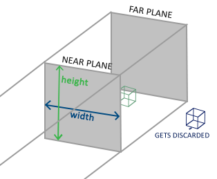
A perspective frustum can be viewed as a non-uniformly shaped box, where every coordinate inside this box will be mapped to a point in clip space. Below is an image of a perspective frustum: 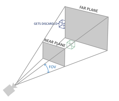If we need a near-far effect, we need to use perspective projection. This projection matrix maps the given frustum range to clip space, and in addition, it modifies the w value of each vertex coordinate so that the w component of vertices farther from the observer becomes larger. Coordinates transformed into clip space will fall within the range of -w to w (any coordinates greater than this range will be clipped). OpenGL requires all visible coordinates to fall within the range of -1.0 to 1.0 as the final output of the vertex shader. Therefore, once coordinates are in clip space, perspective division will be applied to the clip space coordinates:

Each component of the vertex coordinates will be divided by its w component, making the vertex coordinates smaller the farther they are from the observer. This is another reason why the w component is important; it helps us perform perspective projection. The final result coordinates will be in normalized device space.

LookAt

One of the benefits of using matrices is that if you define a coordinate space using three mutually perpendicular (or non-linear) axes, you can create a matrix using these three axes along with a translation vector, and you can multiply this matrix by any vector to transform it into that coordinate space. This is exactly what the LookAt matrix does. Now that we have three mutually perpendicular axes and a position vector defining the camera space, we can create our own LookAt matrix:

Where R is the right vector, U is the up vector, D is the direction vector, and P is the camera position vector. Note that the position vector is negated because we ultimately want to translate the world in the opposite direction of our movement. Using this LookAt matrix as the view matrix can efficiently transform all world coordinates into the just-defined view space. The LookAt matrix does exactly what its name implies: it creates a view matrix that looks at a given target.

A special type of view matrix that creates a coordinate system where all coordinates are rotated or translated based on the user observing the target from a position.

Euler Angles

Defined as Yaw, Pitch, and Roll, allowing us to construct any 3D direction using these three values.